M 57 - Luminance Vs Infrared

Contents

  1. Infrared Imaging

  2. Image Acquisition

  3. Subtracting the Dark Noise

  4. Comparison of Luminance and Infrared Light

An earlier post was of a quick M 57 image in Luminance filter (400 nm-700 nm). In my archives i found a three years old data of this nebula which i did not process at the time.. why do i do it with a lot of my data.. is a mystery to me too :)

Infrared Imaging

It was imaged with an Infrared filter.. yes infrared!! Could’t believe i would even attempt it in the first place!

The filter is Astronomik IR Pro 807 which has a bandpass way above 700 nm. So this will show the invisible light only to the CCD chip. Problem with that is the CCD Quantum Efficiency declines in that band. I use SBIG ST9XE CCD and you can see the QE is quite low in that IR region. At 800 nm, only 45 percent remains.

Celestron C14’s big aperture was a hopeful thing i have.. since it will be able to collect more photons which are coming in a rare quantity from M 57 Ring Nebula.

IR Pro transmission.png

Figure 1. Astronomik IR Pro Specturm

ST9 QE.png

Figure 2. SBIG ST9XE QE Graph

Image Acquisition

Now to image in this very faint light, i decided to expose the camera for 10 minutes. For autoguiding the mount, i found a star bright enough to give my mount one correction every 3 seconds. Pressed the Take Image button and waited for 10 minutes. Will any sign of Ring Nebula show up at my screen?

 
RAW Single IR Pro .png
 

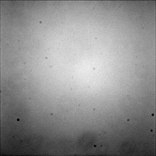
Figure 3. 10 Minutes Raw Image with IR filter

This was the image that came up at my screen.. some random stars and lots of dark noise. Do you see anything else there? any hint of Ring Nebula?

Just in the center, i thought something related to a ring nebula is there.. or is it?

Subtracting the Dark Noise

Since there is so much noise there in Raw image.. I should subtract the dark data from this image and that probably will confirm me if there is the Ring Nebula there or not.

There you go folks.. Ring Nebula in Infrared light!!! It is very dim but can be identified in Figure 4.

Calibrated-Single--M57-IR-Pro.png

Figure 4. Calibrated image of Ring Nebula in IR

Comparison of Luminance and Infrared Light

So i thought to compare the IR image (Figure 5 a) with Luminance image (Figure 5 b). Luminance is what your eyes can see.. 400 nm to 700 nm. Infrared image should show more stars.. Following are the inverted images.. sometimes it is useful to see Astronomical images in inverted frames.

How do you compare these images?

M57-IR-Pro-Cropped Final.png

Figure 5 a. M57 in IR band (Above 807 nm )

M57-L-Cropped Final.png

Figure 5 b. M57 (400 nm - 700 nm)

CCD Linearity Test

Contents

  1. CCD Basics

  2. Rain Drops in Buckets Analogy

  3. CCD’s Linear Relationship

  4. Why Linearity is Important?

  5. Testing My CCD Linearity

  6. Linearity Test Results

There is nothing simpler than using your camera in your phone.. Just open the app with a click and press a button.. or show your hand. That’s it! You have a picture.. Congratulations!

Beneath this process is such a complex amount of science happening in your hand that it would take many many courses to understand it all. So let’s start your first course.. pay attention now!

Kidding :) First, i have very little idea how that happens, except some very basic knowledge.. second, you will runaway from this blog forever and miss all the good things happening here.

So let’s keep it simple here..

CCD Basics

CCD are made of ‘Picture Elements’ or Pixels. These are very small in size and getting smaller with every new chips being produced. You talk about them all the time.. like ‘my camera is 12 Mega Pixels’ etc.. That’s the total number of pixels in your chip which is in your camera. How big can your print of your picture be or how much you can zoom in before you start seeing pixels, that depends on how many pixels you have in your chip.

Almost all of the imaging devices have CMOS chips in them.. This is a different technology and getting better everyday because of the massive demand in the world. But traditionally CCDs have been used for very light sensitive scientific work. Though it seems CCDs are not the future, most of the astroimagers, for now, still have CCDs in their astroimaging cameras. Specially those who wants to have scientifically reliable data.

Light particles (photons) are coming from the stars, galaxies, nebulae, planets, asteroids, comets, background stars and galaxies (which cannot be distinguished in our images), our atmosphere, ground light being reflected by the atmosphere (what did i miss here.. Alien ships?). These photons are directed to our CCDs by our optical systems (telescopes of all kinds and sizes). Next, these light particles are converted into electron and then collected in pixels from where they can be counted when an image is read.

Rain Drops in Buckets Analogy

The analogy (Figure 1), they give us of pixels capturing photons is of buckets catching rain drops.. this is not a bad one and we do get to visualise how the process really happens.

Every pixel is an empty bucket and can gather photons coming from the optical system in the form of electrons. These electrons will be counted, as best as it can be by the camera and as far as physics allows it.

Figure 1. Rainfall Analogy

Nikon Instrument Website

So now the question is.. How many electrons will be generated by the imaging chip, for how many photons it receives. This is called the Quantum Efficiency of the chip.. higher the better.. but it can never be 100%.

Next, suppose if the chip is exposed for one second and it receives 100 photon which results in generating 80 electrons.. that’s a QE of 80%… So far so good.

CCD’s Linear Relationship

But what if i expose it to 2 seconds? It should receive 200 photons and it should generate 160 electron. Doubling the exposure is doubling the electrons.. this is a linear trend and is generating a reliable scientific data.

Like everything else, this does not actually happens in the imaging chips and these devices loose linear relationship at some point. That is the reason why astroimagers are always told to expose the imaging chips to somewhere around half the saturation levels. That will be around 30,000 ADUs. So our data needs to peak at this value and not more than that… or does it?

Linearity test can be done with any imaging chip. You can do it with your DSLR as well. Here i tested my camera. The idea is to start an exposure and keep doubling the exposure time with every next image. Then see if the ADU values are doubling or not? and if this value is doubling, to which ADU range this trend continues.

Why Linearity is Important?

Why it is important to have a linear response? Let’s see a simple example.

Mag-comp.png

Photometry is a technique where we measure one star’s magnitude‘s by comparing an other’s whose magnitude is already knows with some accuracy.

Figure 2. shows an illustration where different stars are shown. Bigger the size, brighter the stars hence lower the magnitude numbers. Yes magnitude system seems confusing at first!

Figure 2. An illustration of Stars in an Image

Suppose we want to measure magnitude of Star B, which seems to be a moderately bright star. Long exposing this star field will produce more ADU numbers for all stars and Star A most probably will leave linear ADU count. Which means Star A can have 30,000 ADU in 30 seconds and 45,000 ADU in 60 seconds (it should be 60,000 ADU for a scientifically useful data), while Star B will double its ADU value from let’s say 5,000 to 10,000 with doubling the exposure time.

Take away lesson: We cannot use ADU value of Star A to find ADU value of Star B in this example. Star C can be a right comparison star here.

I hope now you see the critical importance of linear response needed for any reliable data coming from imaging chips. Those who do the ‘pretty pictures’ work, are doing great but adjusting the ‘curve’ in Photoshop destroys any scientific value of an astronomical image.

Testing My CCD Linearity

I slewed my telescope in the sky trying to find a patch of the sky where stars will not clearly saturate my CCD and also will not be very dim. So for me a part i found was centered here at:

Center RA (2000.0): 17h 23m 09.12s

Center Dec (2000.0): +37° 12' 39.0"

I started my exposure with this sequence of exposure times: 1, 2, 4, 8, 16, 32, 64, 128, 256, 512, 1024 seconds.. doubling the exposure time with every next image and hoping to get double the ADU values.

Image Scale: 0.9470 arcseconds/pixel

Angular/Area Size: 0° 08' 05" x 0° 08' 05"

Position Angle of the CCD camera: 115° 13' from North through East

Figure 3. The chosen star field and the four stars used to measure Linearity of the SBIG CCD

Table 1. shows the exposure values of 11 exposures and the ADU values of four stars marked in Figure 3.

All the images were calibrated with Bias and Dark frames. Dark frames were not taken from the dark frames library but rather taken fresh with matching exposure time of the Raw frames.

Notice with one second exposure, the ADU value is the lowest and increases with increasing exposure time. Now we need to plot this.

Linearity Table Image.png

Table 1. Exposure time vs ADU values of four stars

Linearity Test Results

Figure 4. shows the graph of this comparison. Look at that.. almost surprising result. The CCD is linear to the very end of pixel saturation level. The ‘grey’ star has a bump in the linear line and i do not know why that happened.. could be a cosmic ray hit that could not be corrected with calibration? or is it something else? I am not sure.

But the other stars show a very very linear response.. this is a happy news. This means i can expose my CCD beyond 60,000 counts and still my data will have scientific value. I can accommodate brighter stars in my images and rely on them for good photometric analysis.

There is a reason why Anti Blooming Gate technology is NOT preferred for scientific CCDs.. and mine is a Non Anti Blooming Gate CCD… happy me :)

Figure 4. Exposure time vs ADU count

Asteroid Metis Multiband Flux Comparison

Contents

  1. Asteroid Metis

  2. Multiband Imaging

  3. Asteroid Light Flux

  4. Image Acquisition

  5. Exposure Decision

  6. Results and Analysis

Asteroid Metis

Discovered by Andrew Graham on 25 April 1848, “Metis  is one of the larger main belt asteroid. It is composed of silicates and metallic nickel-iron, and may be the core remnant of a large asteroid that was destroyed by an ancient collision. Metis is estimated to contain just under half a percent of the total mass of the asteroid belt.” (Wikipedia)

“It has the dimensions of 222*182*130 km. Hubble Space Telescope’s images and lightcurve analysis are in agreement that Metis has an irregular elongated shape with one pointed and one broad end. It appears to be more dense than most other asteroids with a diameter close to 200 km. “ (Sky Safari Pro)


Figure 1. Asteroid 9 Metis “Lightcurve based 3D-model” Wikipedia


Multiband Imaging

A few months ago, i imaged this asteroid at my observatory and since it is very bright, i thought to try a multiband imaging with photometric filters i have in my filter wheel. The filters are from Astrodon Company and these are B, V and I (Blue, Visual, Infrared).

Figure 2. Astrodon Photometric Filters Transmittance

Figure 2 a. SBIG ST9XE Quantum Efficiency VS Wavelengths

You can see Astrodon filters bandpass here. There is an overlap of some 25% at 490nm of B and V filter. I filter is nicely separated from B and V but has an overlap of about 40% of 150 nm wavelengths. My CCD has low QE (CCD response for incident photons) in B and I band but high in V band. Which simply means, i would be requiring more exposure for equal amount of flux sources.

Asteroid Light Flux

Since asteroids are much cooler objects in the solar system, their light peaks in Infrared band. Somewhere around 2500-5000 nm. Now i cannot possibly imagine to image at these wavelengths because my filter transmission ends sharply at 900 nm.

But i was hoping to see the brighter asteroid in I band among all of my three photometric bands.. but had no idea how it will actually turn out to be.. needed to experiment on this and see it with my own eyes.

Image Acquisition

Sky X software found the asteroid in no time.. and in the software i found quite a bright star near the target asteroid. The red circle is the asteroid’s position and it is very near to a bright star.

Since the asteroid is very bright, at just over 9 magnitude, i decided to do the unguided imaging with my telescope.

Next step: Deciding the exposure time.


Figure 3. Asteroid Metis Position in Sky X Image

Exposure decision

ADU value is the number which represents the QE of the photon count per pixel. I needed to keep it in 30k range so it does not become non linear. By exposing the camera with different time and keeping an eye on the maximum ADU count for all three BVI filters, i was ready to start my imaging run.

Results and Analysis

So have a look at the following images and their respective graphs.. what do you make out of these? You can comment down there.. Let’s analyze it together :)

Figure 4. Metis (B band)

Figure 4 a. Flux Graph (B band)

Figure 5. Metis (V band)

Figure 5 a. Flux Graph (V band)

Figure 6. Metis (I band)

Figure 6 a. Flux Graph (I band)

Figure 7. Metis (L filter 400-700 nm)

Figure 7 a. Flux graph (L band)

A comparison was made between the maximum flux of the asteroid Metis and the closest bright star.. here is the result. What will be your favorite band to image an asteroid?

Figure 8. Intensity Comparison Graph

M 57 - Playing with the Images

Contents

  1. Images with Graphs

  2. Sky Background

  3. CCD Camera & Telescope Unwanted Noise/Signal

  4. Read Noise

  5. Dark Frame

  6. Flat Frame

  7. Calibrated Result

Images and Graphs

The previous post was about M 57, the famous Ring Nebula.. Let’s play some more here with the images we have.

For our eyes, it is very difficult to compare or measure the light sources such as stars by just looking at an image. All we see is the black background and a bunch of white dots. some are bright some are dim but no real comparison of how much is the difference. Maxim DL has a wonderful feature where it graphs the light quantity or flux of the image, creating a beautiful visualization in 3D.

Figure 1, is the single 300 seconds raw image directly out of the camera. Raw means it has the light of the stars and the Ring Nebula which we want to image but it also has all kinds of unwanted light which we collectively call noise in the image. More about the noise later.

Figure 2, is the intensity graph of the selected area around the Ring Nebula. The darker colors represent low photon (light particles) counts and the brighter ones are the areas where more light has been detected in the image.

Raw 5 min Sub M57.png

Figure 1. 300 seconds RAW Image (faulty auto guiding/tracking making the stars oval instead of round)

Figure 2. Light intensity 3D Graph (Maxim DL)

The deep blue color at the bottom (Figure 2) is the representation of the lowest light detection in the image, which you might think should be zero because the image is from space and well.. space is all black! But the reality is quite different when it comes to imaging the night sky.

Sky Background

The observatory is in Lahore, a heavily light and dust polluted sky always dominates here. On the day of imaging (May 3, 2020), there was moon in the sky, at 80% illumination which was sending all the unneeded photons in the sky and making it anything but dark. So this all moved the background '‘black’ sky floor to higher levels. Astrophotographers try their best to keep this background as low as possible and there are various gadgets and techniques to do that but this can never be zero or rather i should say, should not be zero because then there is no statistical data in that pixel and it will not behave properly when calibrating (cleaning the image) the image begins. A non zero ADU value is very important to have in your pixel!

If you think this is bad enough, nature has other ways to mess up poor astronomers’ lives!

CCD Camera & Telescope Unwanted Noise/Signal

CCD Camera has two noise sources:

  1. Read/BIAS Noise

    When the chip is read, it adds noise in the measurement which is called the read out noise. So what we do is to record the readout noise and then subtract it from the original raw image.

  2. Dark Noise

    At any temperature, photons are produced in the chip. By cooling the CCD chip, we can reduce the number of photons which gets us closer to the wanted signal of the celestial object.

Read Noise

Figure 3 is the Readout Noise image from the camera and Figure 4 shows the 3D graph of this noise. You can see the noise floor is low, 900 some ADU (Analogue to Digital Unit) value. This will be subtracted from the raw image. Bias pixels show less than 1000 ADU values and this value depends on the camera manufacturer.

Some spikes can be seen in Figure 4. This is because not all pixels are created equal. All pixels give a bit different value but some show much higher values than majority of them. These higher values are corrected in the calibration process.

Figure 3. BIAS frame (a zero second exposure is read from the camera)

Figure 4. 3D graph of the BIAS noise

Figure 5 shows the cursor at a pixel which is located at X=391, Y=358 position on the CCD chip and is showing an ADU value of 2264, which can be read at the bottom in the picture. The average pixel value in the Bias frame is 964.

IMG_8235.JPG

Figure 5. Cursor is at bright Pixel number (391, 358) in Bias frame

Figure 6. Pixel number (391, 358) in Bias frame

Same pixel (391, 358) in raw Image shows maximum value of 65,535 ADU, the highest a 16 bit can record. Hot pixels do that.. they would hit the higher or highest values. We always try to avoid the ADU values close to the maximum number in our images because CCDs are not linear in that range and no reliable measurements can be done around these values.

But hot pixels can be fixed in a number of ways. One of the method to keep these pixels in lower ADUs is to keep the CCD temperature as low as possible.

Figure 7. Pixel number (391, 358) in Raw Image

Here is an actual example of calibrating the image. In Figure 6, the pixel has a value of 2264 and in Figure 7, the same pixel in the Raw Image has the value of 65535. Now if we subtract it, the resultant pixel (Figure 8) shows a reduced value of 63373, a difference of 2162.

Hmm.. shouldn’t it be 2264? because that is the value being subtracted. This happens not with the hot pixel but with other pixels too.. every pixel is about a 100 pixel less than the expected value. There must be an explanation.. I have no idea what that is.

IMG_8236.JPG

Figure 8. BIAS subtracted Raw image

Dark Frame

Figure 9, is the 300 seconds exposure with the camera shutter closed and the CCD at -10 Celsius temperature. Figure 10 is the graph of this dark frame.

Figure 9. Dark frame 300 seconds at -10 Celsius

Figure 10. Dark Frame 300 seconds (-10 C)

Flat Frame

Light coming from the any optical system such as a telescope is not perfectly evenly distributed and there will be dust particles in the way no matter how much we want to clean our equipment. To solve this problem, astrophotographers take Flat Frames by imaging an even white surface (there are many ways to take the flat frames) and then dividing it from the raw frame.

Figure 11. Flat frame with Luminance filter

Figure 12. Flat frame (L filter)

Calibrated Result

That’s the difference between a Raw and a Calibrated image (Figure 13 & 14).. A 3D Ring Nebula.

Figure 13. Graph of 300 seconds exposure raw frame

Figure 14. Graph of calibrated 300 seconds image

A NEO (Near Earth Object) observed from the Observatory

Contents:

  1. Amor Asteroids

  2. NEO Target Selection

  3. 2001 MK3 Asteroid

  4. Imaging Concerns

  5. Slewing the Telescope

  6. Image Acquisition

  7. Calibration

  8. Stacking

  9. Astrometrica to the Rescue

  10. Near Earth Asteroid Detected!

AMOR ASTEROIDS

Amor class is a group of asteroids that cross the orbit of Mars.. also known as, Earth-grazing asteroids. Close encounter to Earth or Mars can turn Amors into Earth-crossers (Apollo Group). Amor members show a broad variety of compositional types, evidently having originated from several sources. (Oxford Astronomy Dictionary).

NEO Target Selection

On 30 April, 2020, i checked on Minor Planet Center website for targets (which are desirable for the night) for Astrometry (precise positioning of asteroids or comets) from my observatory in Lahore. The following list came up:

MPC website says the observations for this asteroid are desirable now.

2001 MK3 Asteroid

2001 MK3 is an Amor class asteroid which is less than 2 km in size and was 1.1 AU ( 164,600,000 Km) away on April 30, 2020. It orbits the sun every 2.2 years at an average distance of 1.7 AU (Sky Safari Pro Mobile App). One Astronomical Unit is the mean distance of Earth and Sun.

Asteroid 2001 MK3 orbit around the sun. It crosses the path of Mars but not with Earth. (Images from Sky X)

Imaging Concerns

Imaging and detecting faint asteroids is not an easy task from a light polluted city sky. Stars and Deep Sky Object virtually stay where they are in the sky and we can take multiple exposures for hours long and can keep on collecting their light on a few pixels. On the other hand asteroids (and comets) move noticeably in the sky and hence their light is continuously dispersing on pixels across the CCD. The outcome: a single pixels has far less light of a moving asteroid than a ‘fixed’ star in the sky.

Slewing the Telescope

But why not try it and give it a go so i downloaded and updated 2001 MK3 asteroid in The Sky X software.. This is the software i use to control all my equipment at my observatory. The asteroid is in Herculus Constellation and the following image would be my field of view (FOV) according to the software.


2001 MK3 Position in The Sky X Software


The mark of red circle with three dots, is the position of the asteroid in the sky. I slewed the telescope to the target location.. Now i could see the yellow circle (telescope pointing position in Sky X), moving from the home position to the target position on the Sky X software’s planetarium window. I always use ‘Closed Loop Slew’ in Sky X.. it does three things Automatically: Slews to the target, Plate Solves & Notices to error in pointing and then Slews again with the target in dead center. This feature is such a blessing!

Eden Observatory

Remotely controlled Observatory

Celestron C14 Telescope

Losmandy Titan Mount

SBIG Adaptive Optics

SBIG CCD

Astrodon Filters

Optec Rotator Optec Focuser

Primaluce Eagle

System Focal Length: 4400 mm

Telescope at Eden Astronomical Observatory


Plate solved in the Sky X shows the correct position of the telescope view in the Sky X software. Since my Field of View is small (8 x 8 arcminutes), one of my usual concern is: Do i have enough stars in the field which will give me plate solving for a successful Astrometry? Sometimes there are not enough stars and my only choice is to wait till the asteroid crosses another patch of the sky which has more stars.

This time i was lucky and could see many stars..

Imaging initiated!

Image Acquisition

I kept the sub exposure time at 30 seconds so i could keep the asteroid at one spot. Following is the first image from the telescope.


Single 30 seconds exposure in Luminance filter


Calibration

I took some 65 images. Now need to ‘clean’ these images.. a process which is called Calibrating the Raw. There are various sources of noise in the raw images coming from the camera. Calibration helps a lot in clearing up this noise. There are many sources on the web where this cleaning process is explained so i wont go in these details here.

Calibration Frames: BIAS, DARK and FLAT


Calibrated Image


After calibration, we can see some dim stars as well and an even background.

Stacking

Next step is to Stack or combine all images and let’s find out if the asteroid is visible in the stacked image. Stacked image improves Signal to Noise ratio a lot, which simply means the dim objects become brighter.

 
All Combined 2001 MK3.png

All 65 images combined, created this image.


For those who do not know, telescopes not only need accurate tracking of the sky (due to planet Earth’s rotation around its axis), telescopes also need guiding as well because no tracking is perfect. Here in this imaging run i was not guiding the telescope.. hence the stacking error on the left side.

The combined image showed nothing at the location of the asteroid. Not good!

But i knew the asteroid is very dim against my bright background of city sky and the photons coming out from it will be there in my image somewhere. Since it is moving, i would be need another technique.. a very clever technique indeed!

Astrometrica to the Rescue

Astrometrica is a great software for asteroid trackers. It is simple yet quite powerful to locate an asteroid and find its exact position in the sky.

One of the great feature it has is, it will download an asteroid’s speed, position, the angle in the sky in which it is moving and then it will stack the whole set of images keeping that moving asteroid at one point. This looks pure magic to me!

Following is what Astrometrica retrieved. You can see 2001 MK3 was moving at 0.710 arcseconds per min and with 91 degree position angle. My single exposure was 30 seconds and my image scale is almost 1 arcseconds (0.94 to be exact).


2001 MK3 speed and position (Astrometrica Software)


Near Earth Asteroid Detected!

Ladies and Gents.. 2001 MK3 finally detected :) and right where it is supposed to be! The red box is the position where Astrometrica shows this asteroid should be. The stars trail as expected. Signal to noise Ratio (SNR) is 14 which is not that bad since i only have to know the exact position.

2001 MK3 exact position in the final image (Astrometrica Software)


The 3D flux graph shows the raised position where this asteroid is. Rising above the background noise.

This is my first Near Earth Asteroid detection.. many more would be coming! As far as i know, this is also the first detection of NEO from Pakistan.